North Indian Ocean cyclone climatology#
This notebook explores the full IMD best-track record (1982–present) the way you might with tropycal for other basins: we map every track, look at where storms form, and build a climatology of frequency, seasonality, and intensity for the two North Indian Ocean sub-basins — the Bay of Bengal (BoB) and the Arabian Sea (ARB).
Everything runs against the dataset committed in the repo, so the numbers and
figures below are real and regenerate on every docs build. We load it through
.clean(fix_dates=True) to drop the few QC-flagged coordinate spikes and
correct day/month-transposed dates before analysing.
import matplotlib.pyplot as plt
import numpy as np

import imdtrack as imd

# ---- A small, consistent visual system -----------------------------------
# Two sub-basins are an *identity* (categorical) encoding: one fixed hue each,
# from a colourblind-safe pair (blue vs orange, ΔE well clear of the CVD floor).
# Continuous intensity uses a single perceptually-uniform sequential map (viridis
# — never a rainbow like jet/turbo). Text and chrome stay in neutral ink so the
# colour only ever carries the sub-basin identity.
BOB, ARB, OTHER = "#2a78d6", "#eb6834", "#b8b6ae"
INK, INK2, MUTED, GRID, AXIS = "#0b0b0b", "#52514e", "#898781", "#e1e0d9", "#c3c2b7"
SEQ = "viridis"
BASIN_COLORS = {"BOB": BOB, "ARB": ARB, "LAND": OTHER}
BASIN_NAME = {"BOB": "Bay of Bengal", "ARB": "Arabian Sea", "LAND": "Land"}

plt.rcParams.update(
    {
        "figure.dpi": 120,
        "savefig.bbox": "tight",
        "font.size": 11,
        "axes.titlesize": 13,
        "axes.titleweight": "bold",
        "axes.titlepad": 10,
        "axes.titlecolor": INK,
        "axes.labelsize": 10.5,
        "axes.labelcolor": INK2,
        "axes.edgecolor": AXIS,
        "axes.linewidth": 0.8,
        "axes.grid": True,
        "axes.axisbelow": True,
        "axes.spines.top": False,
        "axes.spines.right": False,
        "grid.color": GRID,
        "grid.linewidth": 0.8,
        "xtick.color": MUTED,
        "ytick.color": MUTED,
        "xtick.labelcolor": INK2,
        "ytick.labelcolor": INK2,
        "text.color": INK,
        "figure.facecolor": "white",
        "axes.facecolor": "white",
        "legend.frameon": False,
        "legend.fontsize": 10,
    }
)


def storm_label(row):
    """A display name, falling back to the storm id for unnamed systems."""
    name = row["name"]
    return name if isinstance(name, str) and name else row["storm_id"]


# Load and clean: drop the handful of coordinate spikes (`pos_suspect`) and fix
# day/month-transposed dates (`date_suspect`) so the map has no impossible jumps
# and genesis months are correct (e.g. Nargis returns to May instead of January).
bt = imd.load().clean(fix_dates=True)
obs = bt.observations.copy()
storms = bt.storms.copy()
bt
Matplotlib is building the font cache; this may take a moment.
<BestTracks: 428 storms, 7569 fixes, 1982-2026>
Headline numbers#
n_storms = len(storms)
yr_min, yr_max = int(storms["year"].min()), int(storms["year"].max())
by_basin = storms["basin"].value_counts()
strongest = storms.loc[storms["max_wind"].idxmax()]

print(f"Record: {n_storms} systems, {yr_min}–{yr_max}")
print(f"By sub-basin: {by_basin.to_dict()}")
print(
    f"Bay of Bengal share: {by_basin.get('BOB', 0) / n_storms:.0%}  |  "
    f"Arabian Sea share: {by_basin.get('ARB', 0) / n_storms:.0%}"
)
print(
    f"Strongest system: {storm_label(strongest)} ({strongest['storm_id']}), "
    f"peak {strongest['max_wind']:.0f} kt, min pressure {strongest['min_pressure']:.0f} hPa"
)
Record: 428 systems, 1982–2026
By sub-basin: {'BOB': 294, 'ARB': 98, 'LAND': 36}
Bay of Bengal share: 69%  |  Arabian Sea share: 23%
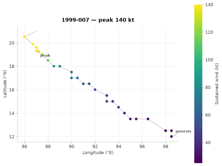
Strongest system: 1999-007 (1999-007), peak 140 kt, min pressure 912 hPa
The Bay of Bengal produces the large majority of North Indian Ocean systems — it is warmer, more humid, and its geometry funnels storms onto densely populated coasts. The Arabian Sea is quieter, but, as we’ll see, its activity has not been steady over time.
Every track on one map#
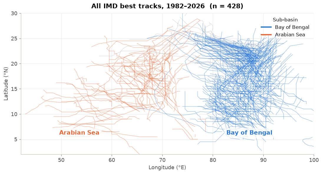
Each line is one storm, coloured by its sub-basin. Even without coastlines the shape of the basin is clear: Bay of Bengal tracks (blue) curve up toward the north-east Indian and Bangladesh coasts, while Arabian Sea tracks (orange) sit to the west.
storm_basin = storms.set_index("storm_id")["basin"]

fig, ax = plt.subplots(figsize=(9, 5.8), layout="constrained")
for sid, g in obs.groupby("storm_id", sort=False):
    ax.plot(
        g["lon"],
        g["lat"],
        color=BASIN_COLORS.get(storm_basin.get(sid), OTHER),
        lw=0.8,
        alpha=0.45,
        solid_capstyle="round",
    )

# Frame the basin (a lone 1989 anomaly aside) so the tracks fill the panel.
ax.set_xlim(42, 100)
ax.set_ylim(2, 30)
ax.set_aspect("equal")

# Region labels sit over their own sub-basin, each on a soft translucent plate
# so it stays legible on top of the tracks; the legend goes top-right, clear of
# both the labels and the dense track cluster.
plate = dict(boxstyle="round,pad=0.35", fc="white", ec="none", alpha=0.72)
ax.text(
    0.20,
    0.14,
    "Arabian Sea",
    transform=ax.transAxes,
    color=ARB,
    fontsize=12,
    fontweight="bold",
    ha="center",
    bbox=plate,
)
ax.text(
    0.78,
    0.14,
    "Bay of Bengal",
    transform=ax.transAxes,
    color=BOB,
    fontsize=12,
    fontweight="bold",
    ha="center",
    bbox=plate,
)

handles = [
    plt.Line2D([], [], color=BASIN_COLORS[b], lw=2.5, label=BASIN_NAME[b])
    for b in ("BOB", "ARB")
    if b in set(storm_basin)
]
ax.legend(handles=handles, loc="upper right", title="Sub-basin", title_fontsize=10)
ax.set_xlabel("Longitude (°E)")
ax.set_ylabel("Latitude (°N)")
ax.set_title(f"All IMD best tracks, {yr_min}–{yr_max}  (n = {n_storms})")
ax.grid(alpha=0.6)
plt.show()
Where do storms form?#
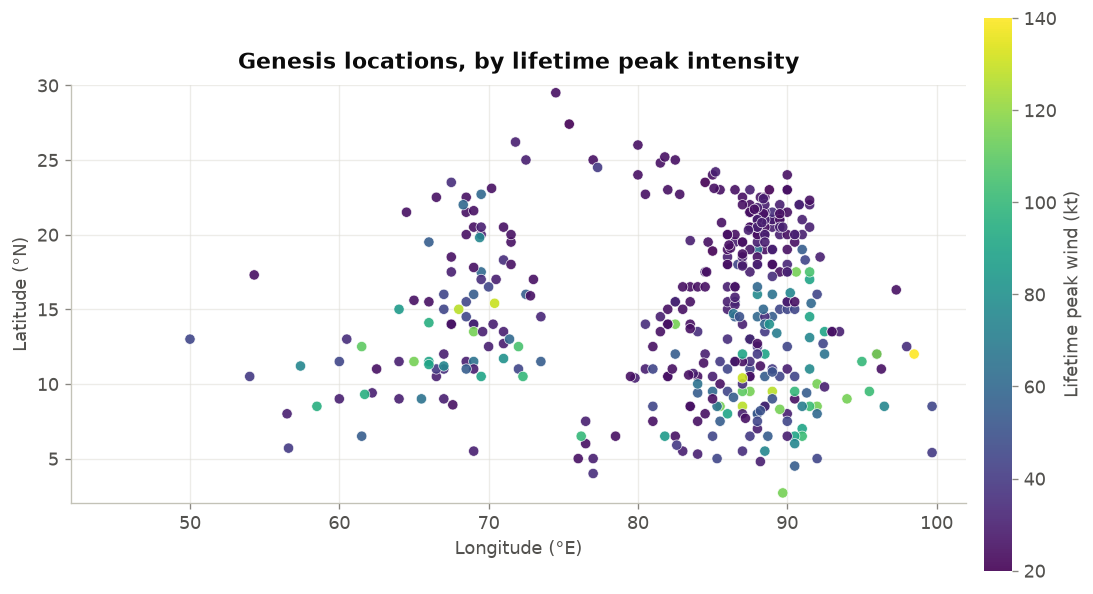
The genesis point is the first fix of each track (step == 0), coloured by
the storm’s lifetime peak wind. The strongest systems tend to originate in the
southern/central Bay of Bengal, with room to intensify before landfall.
genesis = obs[obs["step"] == 0].merge(
    storms[["storm_id", "peak_grade", "max_wind"]], on="storm_id", how="left"
)

fig, ax = plt.subplots(figsize=(9, 5.2), layout="constrained")
sc = ax.scatter(
    genesis["lon"],
    genesis["lat"],
    c=genesis["max_wind"],
    cmap=SEQ,
    s=38,
    alpha=0.9,
    edgecolor="white",
    linewidth=0.4,
)
cb = fig.colorbar(sc, ax=ax, shrink=0.9, pad=0.02)
cb.set_label("Lifetime peak wind (kt)", color=INK2)
cb.outline.set_visible(False)
cb.ax.tick_params(color=MUTED, labelcolor=INK2)
ax.set_xlim(42, 102)
ax.set_ylim(2, 30)
ax.set_aspect("equal")
ax.set_xlabel("Longitude (°E)")
ax.set_ylabel("Latitude (°N)")
ax.set_title("Genesis locations, by lifetime peak intensity")
ax.grid(alpha=0.6)
plt.show()
Annual frequency, split by sub-basin#
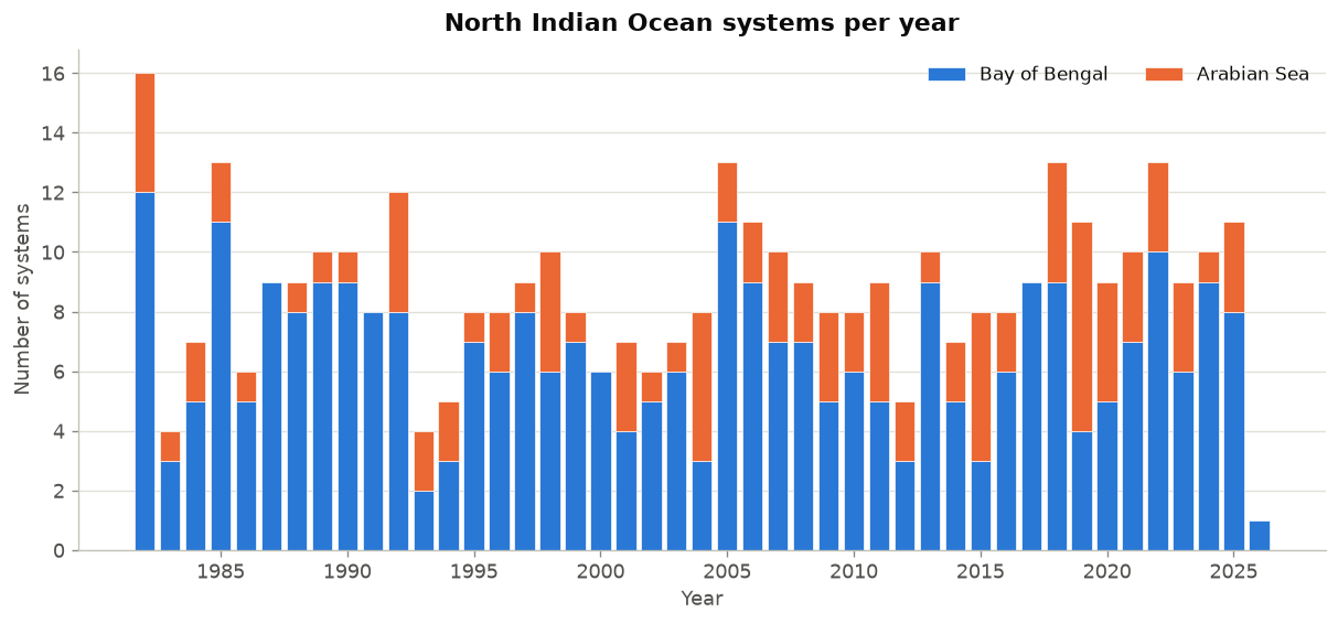
Counts of systems per year. The Bay of Bengal dominates almost every season; the Arabian Sea contributes a smaller, more variable share.
counts = (
    storms.groupby(["year", "basin"], observed=True)
    .size()
    .unstack("basin")
    .reindex(range(yr_min, yr_max + 1), fill_value=0)
)
for col in ("BOB", "ARB"):
    if col not in counts:
        counts[col] = 0

fig, ax = plt.subplots(figsize=(10, 4.6), layout="constrained")
ax.bar(
    counts.index, counts["BOB"], color=BOB, label="Bay of Bengal", edgecolor="white", linewidth=0.4
)
ax.bar(
    counts.index,
    counts["ARB"],
    bottom=counts["BOB"],
    color=ARB,
    label="Arabian Sea",
    edgecolor="white",
    linewidth=0.4,
)
ax.set_xticks([y for y in counts.index if y % 5 == 0])
ax.set_xlabel("Year")
ax.set_ylabel("Number of systems")
ax.set_title("North Indian Ocean systems per year")
ax.grid(axis="x", visible=False)
ax.legend(loc="upper right", ncol=2)
plt.show()
Is the Arabian Sea getting busier?#
A recurring result in the literature is that Arabian Sea activity has increased in recent decades. We can check the record directly by comparing the first and second halves of the period.
mid = (yr_min + yr_max) // 2
early = storms[storms["year"] <= mid]
late = storms[storms["year"] > mid]


def basin_rate(df, basin):
    n_years = df["year"].nunique()
    return (df["basin"] == basin).sum() / n_years if n_years else np.nan


print(
    f"Mean systems per year (ARB):  {yr_min}–{mid}: {basin_rate(early, 'ARB'):.2f}"
    f"   {mid + 1}–{yr_max}: {basin_rate(late, 'ARB'):.2f}"
)
print(
    f"Mean systems per year (BOB):  {yr_min}–{mid}: {basin_rate(early, 'BOB'):.2f}"
    f"   {mid + 1}–{yr_max}: {basin_rate(late, 'BOB'):.2f}"
)
Mean systems per year (ARB):  1982–2004: 1.74   2005–2026: 2.64
Mean systems per year (BOB):  1982–2004: 6.52   2005–2026: 6.55
The double cyclone season#
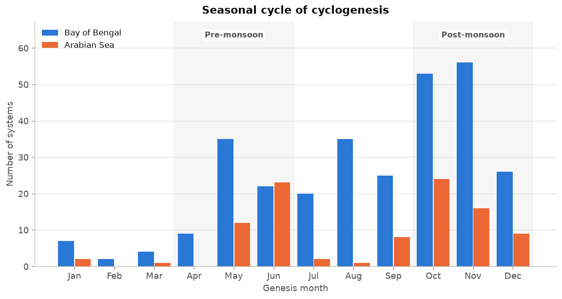
Unlike most basins, the North Indian Ocean has a bimodal season: the summer monsoon suppresses cyclogenesis, leaving two peaks — a pre-monsoon peak (April–June) and a stronger post-monsoon peak (October–December).
gen_month = storms.assign(month=storms["start_time"].dt.month)
season = (
    gen_month.groupby(["month", "basin"], observed=True)
    .size()
    .unstack("basin")
    .reindex(range(1, 13), fill_value=0)
)
for col in ("BOB", "ARB"):
    if col not in season:
        season[col] = 0

months = ["Jan", "Feb", "Mar", "Apr", "May", "Jun", "Jul", "Aug", "Sep", "Oct", "Nov", "Dec"]
x = np.arange(12)
fig, ax = plt.subplots(figsize=(9.5, 5.0), layout="constrained")
ax.bar(x - 0.21, season["BOB"], width=0.4, color=BOB, label="Bay of Bengal")
ax.bar(x + 0.21, season["ARB"], width=0.4, color=ARB, label="Arabian Sea")
ax.margins(y=0.20)  # headroom so the season labels sit clear of the tallest bars

# Shade the two active seasons; label each *inside* the panel near the top (below
# the title, above the bars) so nothing collides.
xtr = ax.get_xaxis_transform()
plate = dict(boxstyle="round,pad=0.3", fc="white", ec="none", alpha=0.75)
for lo, hi, name in [(2.5, 5.5, "Pre-monsoon"), (8.5, 11.5, "Post-monsoon")]:
    ax.axvspan(lo, hi, color=MUTED, alpha=0.07, zorder=0)
    ax.text(
        (lo + hi) / 2,
        0.96,
        name,
        transform=xtr,
        ha="center",
        va="top",
        fontsize=9.5,
        color=INK2,
        fontweight="bold",
        bbox=plate,
    )

ax.set_xticks(x)
ax.set_xticklabels(months)
ax.set_xlabel("Genesis month")
ax.set_ylabel("Number of systems")
ax.set_title("Seasonal cycle of cyclogenesis")
ax.grid(axis="x", visible=False)
ax.legend(loc="upper left", ncol=1)
plt.show()
Intensity distribution#
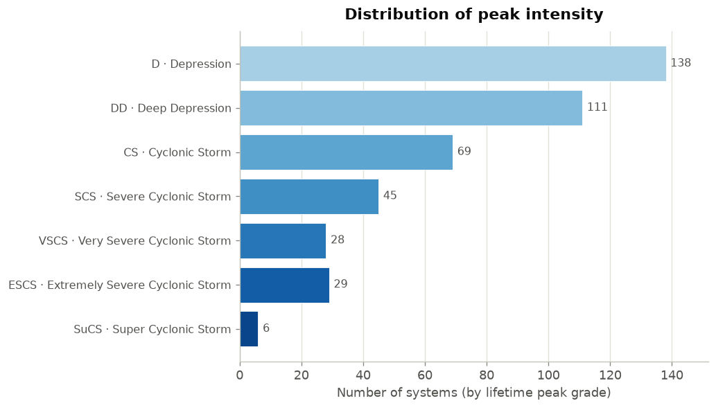
IMD grades systems on an ordered scale from Depression (D) to Super Cyclonic
Storm (SuCS). Most never get past Cyclonic Storm; only a handful each decade
reach the top categories. A horizontal layout keeps the category names readable
and the counts labelled directly.
from imdtrack import GRADE_LONG, GRADE_ORDER  # noqa: E402

grade_counts = storms["peak_grade"].value_counts().reindex(GRADE_ORDER, fill_value=0)
# Ordinal shading: weaker grades lighter, stronger darker (implies intensity).
ramp = plt.cm.Blues(np.linspace(0.35, 0.92, len(GRADE_ORDER)))
ypos = np.arange(len(GRADE_ORDER))

fig, ax = plt.subplots(figsize=(8.5, 4.8), layout="constrained")
bars = ax.barh(ypos, grade_counts.values, color=ramp, edgecolor="white", linewidth=0.5)
ax.set_yticks(ypos)
ax.set_yticklabels([f"{g} · {GRADE_LONG[g]}" for g in GRADE_ORDER], fontsize=9.5)
ax.invert_yaxis()  # strongest at the bottom, weakest at top
ax.bar_label(bars, padding=4, color=INK2, fontsize=9.5)
ax.set_xlabel("Number of systems (by lifetime peak grade)")
ax.set_title("Distribution of peak intensity")
ax.grid(axis="y", visible=False)
ax.margins(x=0.10)  # room for the count labels
plt.show()
An ACE-like activity index#
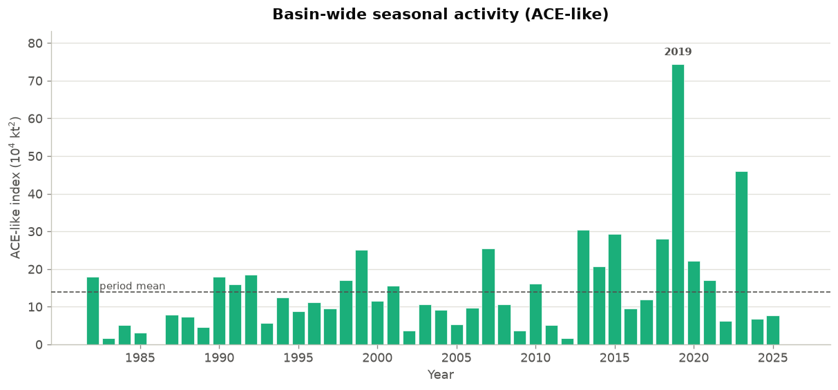
Accumulated Cyclone Energy (ACE) sums the square of the maximum sustained wind over a storm’s life, counting only fixes at tropical-storm strength (≥ 34 kt) at 6-hourly (synoptic) times. The IMD record is 3-hourly, so we subsample to the synoptic hours to approximate the standard definition — treat this as an ACE-like index rather than an official value.
syn = obs[obs["time"].dt.hour.isin([0, 6, 12, 18])]
syn = syn[syn["wind"] >= 34.0]
ace = 1e-4 * (syn["wind"] ** 2)
ace_year = ace.groupby(syn["year"]).sum().reindex(range(yr_min, yr_max + 1), fill_value=0)

fig, ax = plt.subplots(figsize=(10, 4.6), layout="constrained")
ax.bar(ace_year.index, ace_year.values, color="#1baf7a", edgecolor="white", linewidth=0.4)
ax.axhline(ace_year.mean(), color=INK2, ls="--", lw=1, zorder=3)
ax.text(yr_min, ace_year.mean(), "  period mean", va="bottom", ha="left", fontsize=9, color=INK2)

# Label just the single busiest season, offset above its bar (no collisions).
peak_year = int(ace_year.idxmax())
ax.annotate(
    str(peak_year),
    xy=(peak_year, ace_year.loc[peak_year]),
    xytext=(0, 8),
    textcoords="offset points",
    ha="center",
    fontsize=9,
    fontweight="bold",
    color=INK2,
)
ax.set_xticks([y for y in ace_year.index if y % 5 == 0])
ax.set_xlabel("Year")
ax.set_ylabel("ACE-like index (10$^4$ kt$^2$)")
ax.set_title("Basin-wide seasonal activity (ACE-like)")
ax.grid(axis="x", visible=False)
ax.margins(y=0.12)
plt.show()
The strongest storms on record#
top10 = (
    storms.sort_values("max_wind", ascending=False)
    .head(10)[["storm_id", "name", "basin", "start_time", "peak_grade", "max_wind", "min_pressure"]]
    .reset_index(drop=True)
)
top10
| storm_id | name | basin | start_time | peak_grade | max_wind | min_pressure | |
|---|---|---|---|---|---|---|---|
| 0 | 1999-007 | NaN | BOB | 1999-10-25 06:00:00 | SuCS | 140.0 | 912.0 |
| 1 | 2019-007 | KYAAR | ARB | 2019-10-24 03:00:00 | SuCS | 130.0 | 922.0 |
| 2 | 2020-001 | AMPHAN | BOB | 2020-05-16 00:00:00 | SuCS | 130.0 | 920.0 |
| 3 | 1991-001 | NaN | BOB | 1991-04-24 12:00:00 | SuCS | 127.0 | 918.0 |
| 4 | 1990-001 | NaN | BOB | 1990-05-04 06:00:00 | SuCS | 127.0 | 920.0 |
| 5 | 2007-003 | GONU | ARB | 2007-06-01 18:00:00 | SuCS | 127.0 | 920.0 |
| 6 | 2023-002 | MOCHA | BOB | 2023-05-09 12:00:00 | ESCS | 115.0 | 938.0 |
| 7 | 2019-002 | FANI | BOB | 2019-04-26 03:00:00 | ESCS | 115.0 | 932.0 |
| 8 | 1982-001 | NaN | BOB | 1982-05-01 03:00:00 | VSCS | 115.0 | NaN |
| 9 | 2001-001 | NaN | ARB | 2001-05-21 12:00:00 | ESCS | 115.0 | 932.0 |
Track of the most intense system#
Colouring a single track by wind speed shows the classic intensification-then-landfall life cycle. Genesis and lifetime-peak points are marked directly.
track = bt.storm(strongest["storm_id"]).reset_index(drop=True)
peak_i = int(track["wind"].idxmax())

fig, ax = plt.subplots(figsize=(7.5, 6.5), layout="constrained")
ax.plot(track["lon"], track["lat"], color=AXIS, lw=1.2, zorder=0)
sc = ax.scatter(
    track["lon"],
    track["lat"],
    c=track["wind"],
    cmap=SEQ,
    s=48,
    edgecolor="white",
    linewidth=0.4,
    zorder=2,
)
cb = fig.colorbar(sc, ax=ax, shrink=0.85, pad=0.02)
cb.set_label("Sustained wind (kt)", color=INK2)
cb.outline.set_visible(False)
cb.ax.tick_params(color=MUTED, labelcolor=INK2)

for i, tag, dx, dy in [(0, "genesis", 10, 10), (peak_i, "peak", 10, -14)]:
    ax.annotate(
        tag,
        xy=(track["lon"][i], track["lat"][i]),
        xytext=(dx, dy),
        textcoords="offset points",
        fontsize=9,
        color=INK2,
        fontweight="bold",
        arrowprops=dict(arrowstyle="-", color=MUTED, lw=0.8),
    )
ax.set_aspect("equal")
ax.set_xlabel("Longitude (°E)")
ax.set_ylabel("Latitude (°N)")
ax.set_title(f"{storm_label(strongest)} — peak {strongest['max_wind']:.0f} kt")
ax.grid(alpha=0.6)
plt.show()
Takeaways#
The Bay of Bengal dominates North Indian Ocean cyclone activity, but the Arabian Sea is the more variable — and, in this record, increasingly active — sub-basin.
The basin’s defining feature is its bimodal season, split by the summer monsoon into pre- and post-monsoon peaks.
Most systems stay weak; a small tail of intense storms drives the basin-wide ACE-like index and, of course, the impacts.
From here you can slice the xarray view for gridded
analysis, or pull any single storm with bt.storm(...).